import matplotlib
if not hasattr(matplotlib.RcParams, "_get"):
    matplotlib.RcParams._get = dict.get
Generate ERA5 forcing: own shapefile#
This will consist of two parts in separate notebooks:
using a shapefile from Caravan
using your own shapefile!
ERA5 need 4 different inputs:
a shapefile
a time-window
a directory to save the data
and a type of forcing
Using your own shapefile#
If you have your own shapefile, skip the first part. First I will guide your through making your own shapefile!
Make your own shapefile#
There are several ways to make shapefiles:
Make one using Arcgis.
Get the station.json from a GRDC station, which can be converted into a shapefile or multiple if you have a bigger area.
You also need 5 different files:
.shp
.cpg
.prj
.dbf
.shx
We already have these files from the camels, but they are in a different directory now, for the purpose of this notebook
# General python
import warnings
warnings.filterwarnings("ignore", category=UserWarning)

import numpy as np
from pathlib import Path
import pandas as pd
import matplotlib.pyplot as plt
import xarray as xr

# Niceties
from rich import print

# General eWaterCycle
import ewatercycle
import ewatercycle.forcing
# The name of the shapefile
shape_file_name = "camelsgb_33039"  # river: Bedford Ouse at Roxton, England

# The time-window of the experiment
experiment_start_date = "2000-08-01T00:00:00Z"
experiment_end_date = "2005-08-31T00:00:00Z"

# The path save directory of the ERA5 data
forcing_path_ERA5 = Path.home() / "forcing" / shape_file_name / "ERA5" / "own_shapefile"
forcing_path_ERA5.mkdir(exist_ok=True)
Now we just point to where the shapefiles are, but to the .shp file specifically.
# The path to the shapefiles
shapefile_path =  Path.home() / "getting-started/book/some_content/forcing/shapefiles" / f"{shape_file_name}.shp"  # check this directory yourself!
ERA5 Forcing Generation#
Now that we have the shapefile we can almost get the ERA5 forcing. But first we need to define a new path. And we need to pick what kind of forcing we want to generate, this depends on what model you want to use, currently these sources are supported:
LumpedMakkinkForcing
DistributedMakkinkForcing
DistributedUserForcing
GenericDistributedForcing
GenericLumpedForcing
HypeForcing
LisfloodForcing
LumpedUserForcing
MarrmotForcing
PCRGlobWBForcing
WflowForcing
More details can be found in the documentation. And also in the models section.
For now we will use ‘lumped Makkink forcing’, this is needed for running an HBV model.
ERA5_forcing = ewatercycle.forcing.sources["LumpedMakkinkForcing"].generate(
   dataset="ERA5",
   start_time=experiment_start_date,
   end_time=experiment_end_date,
   shape=shapefile_path,
   directory=forcing_path_ERA5,
)
print(ERA5_forcing)
LumpedMakkinkForcing(
    start_time='2000-08-01T00:00:00Z',
    end_time='2005-08-31T00:00:00Z',
    directory=PosixPath('/home/mmelotto/forcing/camelsgb_33039/ERA5/own_shapefile/work/diagnostic/script'),
    shape=PosixPath('/home/mmelotto/getting-started/book/some_content/forcing/shapefiles/camelsgb_33039.shp'),
    filenames={
        'pr': 'OBS6_ERA5_reanaly_1_day_pr_2000-2005.nc',
        'tas': 'OBS6_ERA5_reanaly_1_day_tas_2000-2005.nc',
        'rsds': 'OBS6_ERA5_reanaly_1_day_rsds_2000-2005.nc',
        'evspsblpot': 'Derived_Makkink_evspsblpot.nc'
    }
)
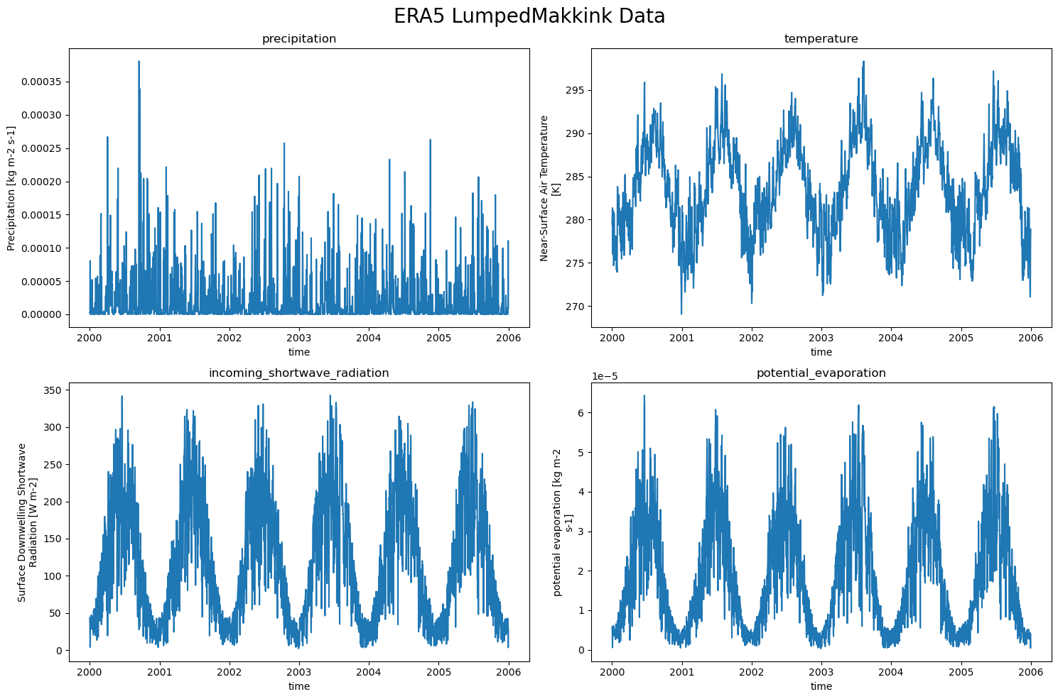
So the LumpedMakkinkForcing stores the following:
pr: precipitation
tas: temperature
rsds: incoming shortwave radiation
evspsblpot: potential evaporation (note that this is calculated, using Makkink)
We can also load the forcing data after we have generated it:
load_location = forcing_path_ERA5 / "work" / "diagnostic" / "script"  # this is needed because the data is stored in a sub-directory
ERA5_forcing = ewatercycle.forcing.sources["LumpedMakkinkForcing"].load(directory=load_location)
print(ERA5_forcing)
LumpedMakkinkForcing(
    start_time='2000-08-01T00:00:00Z',
    end_time='2005-08-31T00:00:00Z',
    directory=PosixPath('/home/mmelotto/forcing/camelsgb_33039/ERA5/own_shapefile/work/diagnostic/script'),
    shape=PosixPath('/home/mmelotto/forcing/camelsgb_33039/ERA5/own_shapefile/work/diagnostic/script/camelsgb_33039
.shp'),
    filenames={
        'pr': 'OBS6_ERA5_reanaly_1_day_pr_2000-2005.nc',
        'tas': 'OBS6_ERA5_reanaly_1_day_tas_2000-2005.nc',
        'rsds': 'OBS6_ERA5_reanaly_1_day_rsds_2000-2005.nc',
        'evspsblpot': 'Derived_Makkink_evspsblpot.nc'
    }
)
The data#
We can easily plot the data now!
ERA5_data = {'precipitation pr': xr.open_dataset(ERA5_forcing['pr']),
             'temperature tas': xr.open_dataset(ERA5_forcing['tas']),
             'incoming_shortwave_radiation rsds': xr.open_dataset(ERA5_forcing['rsds']),
             'potential_evaporation evspsblpot': xr.open_dataset(ERA5_forcing['evspsblpot'])
}

plot_counter = 1
plt.figure(figsize=(15, 10))
for name, data in ERA5_data.items():
    plt.subplot(2,2, plot_counter)
    data[name.split(" ")[-1]].plot()
    plt.title(f"{name.split(" ")[0]}")
    plot_counter += 1

plt.suptitle("ERA5 LumpedMakkink Data", fontsize=20)
plt.tight_layout()