CDF comparison of ERA5 and CMIP model outputs

NOTE this is an adaptation of the full climate change impact analysis (Hut, 2025), changed so it works in this workshop.

By sorting the output in order of decreasing discharge, we can easily make a cummalative distribution. By taking the difference of these functions we derive a (very simple) bias correction function that can later be used to bias-correct the future model output when forced with CMIP projections.

# General python
import warnings
warnings.filterwarnings("ignore", category=UserWarning)

import numpy as np
from pathlib import Path
import pandas as pd
import matplotlib.pyplot as plt
import xarray as xr
import json

# Niceties
from rich import print
from util_functions import create_forcing_data_HBV_from_nc

# General eWaterCycle
import ewatercycle
import ewatercycle.forcing

# For MEV
from scipy.stats import genextreme, gumbel_r, weibull_min

# Load settings
# Read from the JSON file
with open("settings.json", "r") as json_file:
    settings = json.load(json_file)

print(settings)

{
    'country': 'Zimbabwe',
    'caravan_id': 'AF_1491830.0',
    'calibration_start_date': '1961-10-01T00:00:00Z',
    'calibration_end_date': '1978-11-21T00:00:00Z',
    'future_start_date': '2029-08-01T00:00:00Z',
    'future_end_date': '2049-08-31T00:00:00Z',
    'base_path': '/home/mmelotto/my_data/workshop_africa',
    'central_data_path': '/data/shared/climate-data/camels_africa/zimbabwe/camel_data',
    'path_shape': 
'/data/shared/climate-data/camels_africa/zimbabwe/camel_data/shapefiles/AF_1491830/AF_1491830.shp',
    'path_caravan': '/home/mmelotto/my_data/workshop_africa/forcing_data/AF_1491830.0/caravan',
    'path_ERA5': '/home/mmelotto/my_data/workshop_africa/forcing_data/AF_1491830.0/ERA5',
    'path_CMIP6': '/home/mmelotto/my_data/workshop_africa/forcing_data/AF_1491830.0/CMIP6',
    'path_output': '/home/mmelotto/my_data/workshop_africa/output_data/AF_1491830.0',
    'hbv_parameters': [10.0, 0.87, 592.0, 1.4, 0.3, 1.0, 0.09, 0.01, 0.001],
    'SCE_calibration_parameters': [
        6.586012553845907,
        1.0,
        557.8536779504233,
        2.939688843608312,
        0.001,
        1.0,
        0.1,
        0.00024827990873074545,
        3.2087728977063117
    ],
    'monte_carlo_calibration_parameters': [
        2.2809924457194377,
        0.8237298558744328,
        464.7470066408867,
        1.5984658697300798,
        0.29785129445020814,
        1.1825488171931156,
        0.07487754017358864,
        0.008908532718571173,
        5.605800944680686
    ]
}

# Open the output of the historic model and ERA5 runs
xr_historic = xr.open_dataset(Path(settings['path_output']) / (settings['caravan_id'] + '_historic_output.nc'))

print(xr_historic)

<xarray.Dataset> Size: 175kB
Dimensions:                                  (time: 6261)
Coordinates:
  * time                                     (time) datetime64[ns] 50kB 1961-...
Data variables:
    modelled discharge, forcing: historical  (time) float64 50kB ...
    modelled discharge, forcing: ERA5        (time) float64 50kB ...
    Observed Q Caravan                       (time) float32 25kB ...
Attributes:
    units:    mm/d

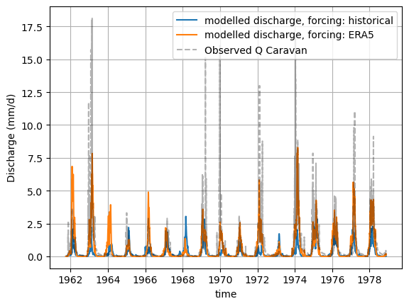
def plot_hydrograph(data_array):
    plt.figure()
    for name, da in data_array.data_vars.items():
        if name == "Observed Q Caravan":
            data_array[name].plot(linestyle='--', color='black', label=name, alpha=0.3)
        else:
            data_array[name].plot(label = name)
    plt.ylabel("Discharge (mm/d)")
    plt.grid()
    plt.legend()


xr_one_year = xr_historic.sel(time=slice('1970-09-01', '1971-08-31'))

plot_hydrograph(xr_historic)
plot_hydrograph(xr_one_year)

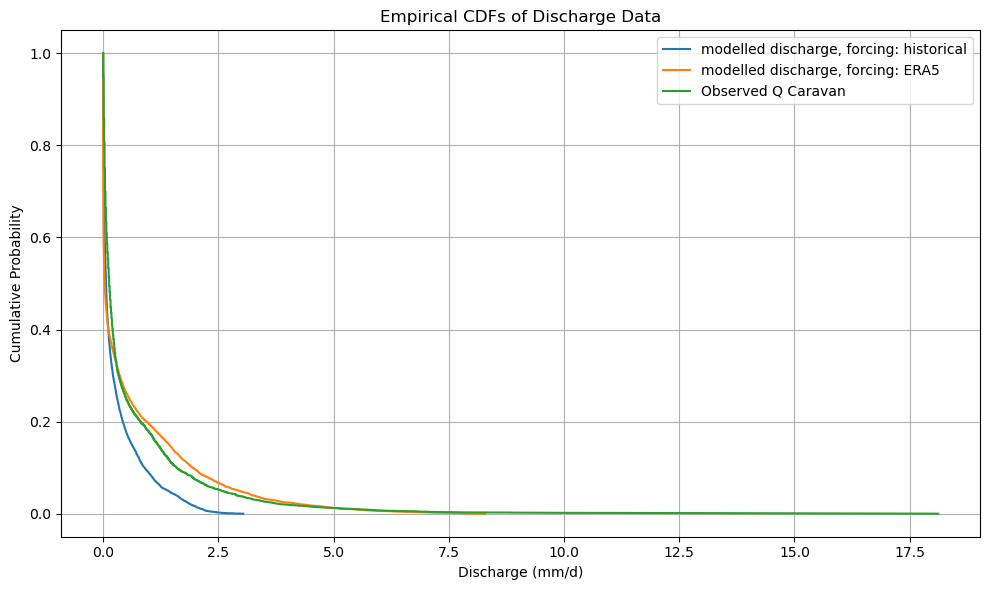
def plot_cdf(ds):
    """
    plot cdf for all data variables 

    Parameters:
    - ds: xarray.Dataset
                       defaults to True
    Returns:
    - nothing
    """
    # 1. Drop time points with missing data in any variable
    valid_ds = ds.dropna(dim="time")
    
    # 2. Sort each variable from highest to lowest
    sorted_vars = {
        name: np.sort(valid_ds[name].values)[::-1]  # sort descending
        for name in valid_ds.data_vars
    }
    
    # 3. Create new indices
    n = len(valid_ds.time)
    cdf_index = np.linspace(0, 1, n)
    return_period_days = np.linspace(n, 1, n)
    return_period_years = return_period_days / 365.25  # convert to years
    
    # 4. Construct new xarray Dataset for CDFs
    cdf_ds = xr.Dataset(
        {
            name: ("cdf", sorted_vars[name])
            for name in sorted_vars
        },
        coords={
            "cdf": cdf_index,
            "return_period": ("cdf", return_period_years)
        }
    )
    
    # 5. Plot the CDFs
    plt.figure(figsize=(10, 6))
    for name in cdf_ds.data_vars:
        plt.plot(cdf_ds[name], cdf_ds.cdf, label=name)
    
    plt.ylabel("Cumulative Probability")
    plt.xlabel("Discharge (mm/d)")
    plt.title("Empirical CDFs of Discharge Data")
    plt.legend()
    plt.grid(True)
    plt.tight_layout()
    plt.show()
    
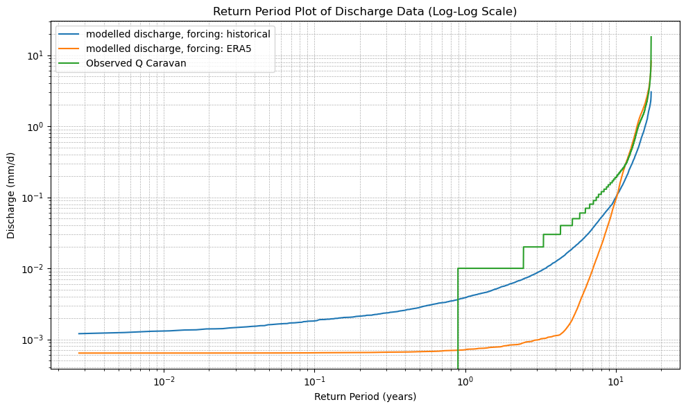
    # 6. Plot the Return Period curves (log-log scale)
    plt.figure(figsize=(10, 6))
    for name in cdf_ds.data_vars:
        plt.plot(cdf_ds.return_period, cdf_ds[name], label=name)
    
    plt.xscale("log")
    plt.yscale("log")
    plt.xlabel("Return Period (years)")
    plt.ylabel("Discharge (mm/d)")
    plt.title("Return Period Plot of Discharge Data (Log-Log Scale)")
    plt.legend()
    plt.grid(True, which="both", linestyle="--", linewidth=0.5)
    plt.tight_layout()
    plt.show()

plot_cdf(xr_historic)

def calculate_mev(ds, dist_type='gev'):
    """
    Calculate MEV-based return periods for all data variables in an xarray.Dataset.

    Parameters:
    - ds: xarray.Dataset
    - dist_type: str, one of ['gev', 'gumbel', 'weibull']

    Returns:
    - xarray.Dataset with MEV return periods
    """
    # Step 1: Drop time points with missing data in any variable
    valid_ds = ds.dropna(dim="time", how="any")

    # Step 2: Extract daily values for each year
    years = np.unique(valid_ds['time.year'].values)
    mev_distributions = {}

    for var in ds.data_vars:
        annual_params = []
        for year in years:
            values = valid_ds[var].sel(time=str(year)).values
            if len(values) > 0:
                # Fit distribution based on dist_type
                if dist_type == 'gev':
                    params = genextreme.fit(values)
                    dist_func = genextreme
                elif dist_type == 'gumbel':
                    params = gumbel_r.fit(values)
                    dist_func = gumbel_r
                elif dist_type == 'weibull':
                    params = weibull_min.fit(values)
                    dist_func = weibull_min
                else:
                    raise ValueError("dist_type must be one of ['gev', 'gumbel', 'weibull']")
                annual_params.append(params)

        # Generate MEV by averaging annual distributions
        x_vals = np.linspace(np.min(valid_ds[var]), np.max(valid_ds[var]), 1000)
        cdfs = [dist_func.cdf(x_vals, *params) for params in annual_params]
        mean_cdf = np.mean(cdfs, axis=0)
        return_period = 1 / (1 - mean_cdf)

        mev_distributions[var] = (x_vals, return_period)

    # Step 3: Create MEV xarray Dataset
    mev_ds = xr.Dataset(
        {
            var: ("x", mev_distributions[var][1])
            for var in mev_distributions
        },
        coords={
            "x": list(mev_distributions.values())[0][0],
        },
        attrs=ds.attrs  # retain metadata
    )

    return mev_ds

def plot_mev(*mev_datasets, dist_type='gev', labels=None):
    """
    Plot MEV curves from one or more xarray.Dataset objects created by calculate_mev().

    Parameters:
    - mev_datasets: one or more xarray.Dataset objects
    - dist_type: str, name of the distribution used (for plot title)
    - labels: list of str, labels for each dataset
    """
    plt.figure(figsize=(10, 6))

    for i, mev_ds in enumerate(mev_datasets):
        prefix = f"{labels[i]} - " if labels else ""
        for var in mev_ds.data_vars:
            plt.plot(mev_ds[var].values, mev_ds['x'].values, label=f"{prefix}{var}")

    plt.xscale("log")
    plt.yscale("log")
    plt.xlabel("Return Period (years)")
    plt.ylabel("Discharge (mm/d)")
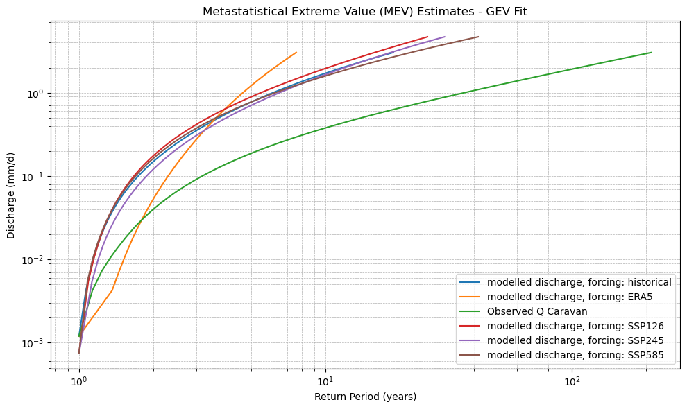
    plt.title(f"Metastatistical Extreme Value (MEV) Estimates - {dist_type.upper()} Fit")
    plt.legend()
    plt.grid(True, which="both", linestyle="--", linewidth=0.5)
    plt.tight_layout()
    plt.show()

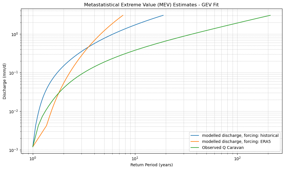
xr_mev_historic = calculate_mev(xr_historic,'weibull')
plot_mev(xr_mev_historic)

# Open the output of the CMIP runs
xr_future = xr.open_dataset(Path(settings['path_output']) / (settings['caravan_id'] + '_future_output.nc'))

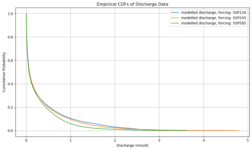
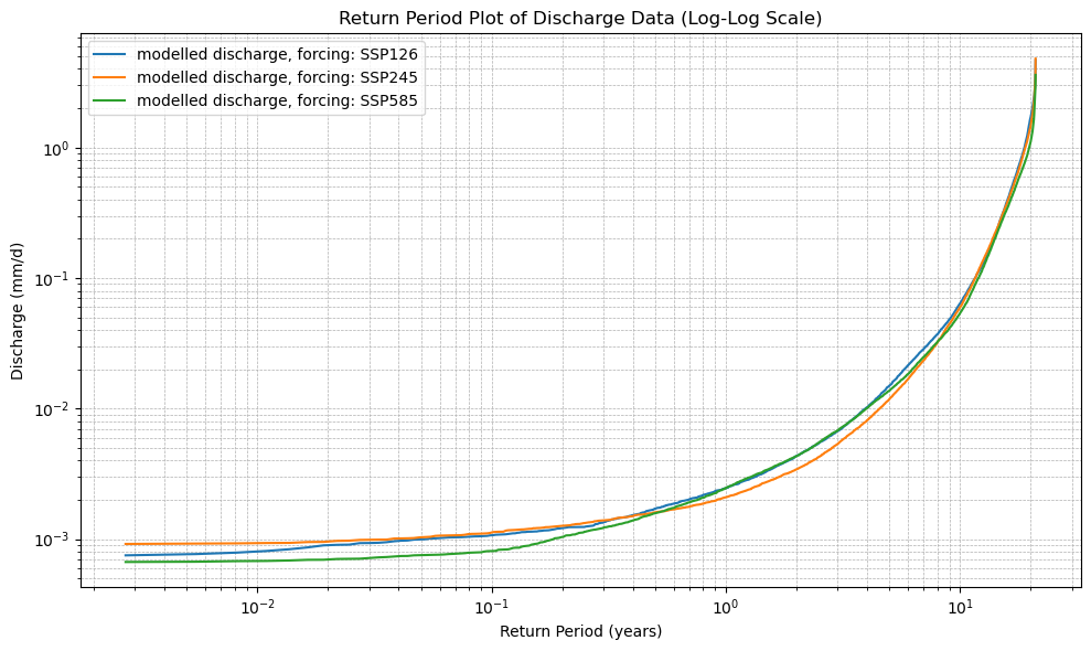
plot_cdf(xr_future)

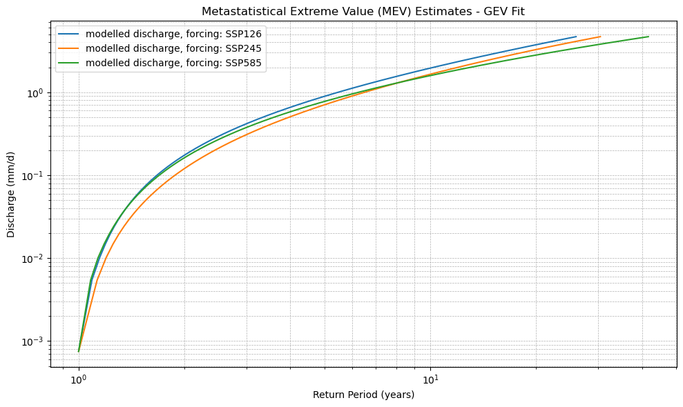
xr_mev_future = calculate_mev(xr_future,'weibull')
plot_mev(xr_mev_future)

plot_mev(xr_mev_historic, xr_mev_future)