Results

This chapter presents the results derived from the methodology outlined in Chapter 2. Using the hydrological model PCR-GlobWB, simulations are conducted to provide insights into the impact of climate change on groundwater recharge. Section 3.1 the historical groundwater recharge and its approximation are simulated to establish a baseline. Section 3.2 focuses on the simulated groundwater recharge, while Section 3.3 focuses on the approximated groundwater recharge. These latter two sections focus on the future climate scenarios.

Historical Groundwater Recharge

To generate a forcing dataset with historical data, an ERA5-dataset spanning the period 1990 to 2020 is used in a generate forcing notebook. The parameter set defines a specific catchment area by defining several coordinates on the ERA5-grid. The outcomes obtained from this forcing dataset and the parameter set in notebooks, the results are simulated (eWaterCycle/projects). This serves as a baseline for evaluating results simulated with CMIP6. Both the groundwater recharge and the approximated groundwater recharge have been analysed and plotted for the 1990-2020 period, as illustrated in Figure 7.

The groundwater recharge depicted in Figure 7 demonstrates relatively low values, with outliers ranging from \(0.024\) to \(0.002\) \(mm/\text{day}\). Comparing the groundwater recharge values to the calculated groundwater recharge from Section 2.5, these values are significantly lower, and do not align with the realistic magnitude of the benchmark established earlier. In contrast, the values of the approximated groundwater recharge are more closely aligned with the magnitude of the benchmark provided in Section 2.5.

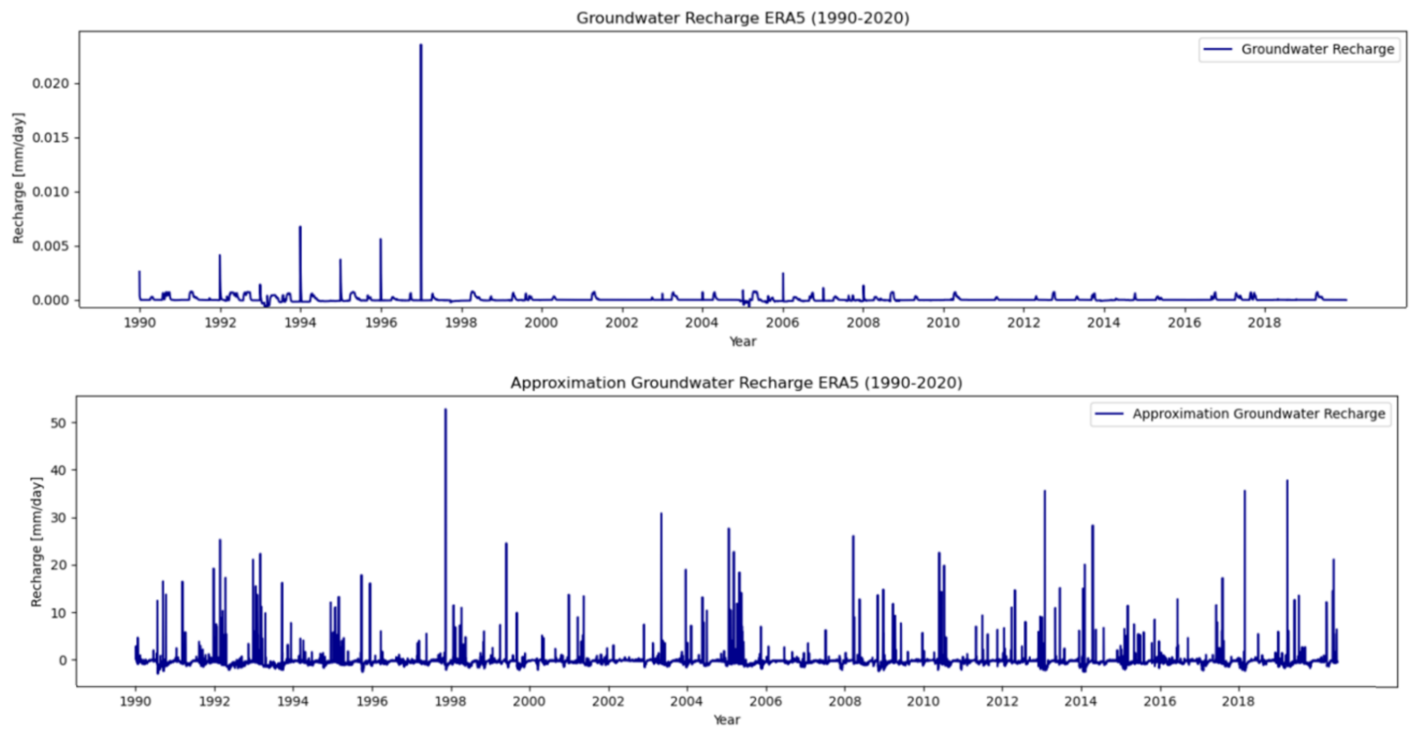Figure 7: Groundwater recharge ERA5 and approximated groundwater recharge ERA5 for period 1990 to 2020.

Figure 8 presents the boxplots for the groundwater recharge and approximated groundwater recharge, highlighting the discrepancy between these values. These boxplots demonstrate that the groundwater recharge values are notably lower than those of the approximated groundwater recharge. Appendix D contains a concise analysis of the outliers in the boxplots. The analysis uses the Z-value to detect and evaluate outliers, based on their standard deviation and mean. The appendix also includes revised boxplots that exclude the outlier, offering a clearer representation of the data.

Figure 8: Boxplots of groundwater recharge ERA5 (left) and approximated groundwater recharge ERA5 (right) over period 1990 to 2020.

Table 2 provides a quantitative summary of the boxplots and the mean summation of groundwater recharge per year. Specifically, the summation of the approximated groundwater recharge, calculated as -123.05 mm, serves as a benchmark for evaluating future climate simulation results in Sections 3.2 and 3.3.

	Groundwater recharge [\(mm/\text{day}\)]	Approximated groundwater recharge [\(mm/\text{day}\)]
Minimum	\(-0.001\)	\( -3.009 \)
Mean	\( 4.961 \)	\( -0.337 \)
Maximum	\( 0.024 \)	\( 52.786 \)
Summation	\( 0.544 \)	\( -123.046 \)

Simulated Groundwater Recharge

The three future climate scenarios are simulated by re-using the established parameter set, and adjusting the CMIP6 grid size to the ERA5 grid size in the generate forcing notebook. This modification accounts for the differing spatial resolution between the ERA5 and CMIP6 dataset.
Three forcing datasets were created for the three SSPs (SSP1-2.6, SSP2-4.5 and SSP5-8.5), covering the period from 2025 to 2100. By applying the generated forcing and the parameter set in notebook, results based on CMIP6 data were obtained.

Figure 9 illustrates the groundwater recharge over the near-term and mid-term period of 2025 to 2065. Outliers in the graph have a small range. These value are consistent with the outcome of Section 3.1 and, once again, do not align with the magnitude of the benchmark set in Section 2.5. To offer further clarity, Figure 10 provides a detailed visual representation of groundwater recharge for the years 2025 and 2050. This figure shows the low groundwater recharge value for a year.

Given that the simulated groundwater recharge values remain significantly smaller than the realistic benchmark magnitude set in Section 2.5, this variable is unrealistic and is unsuitable for further analysis within this study.

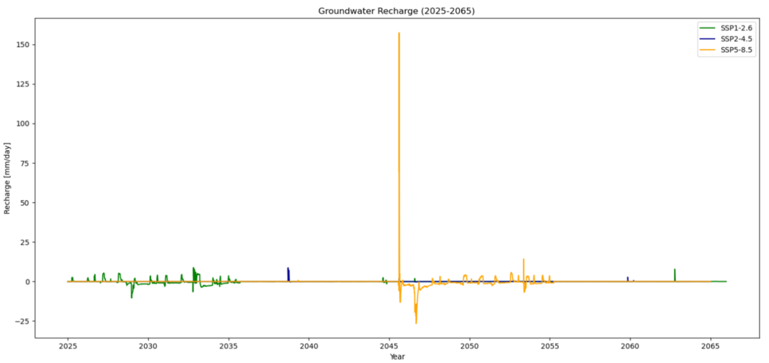Figure 9: Groundwater recharge (2025-2065).

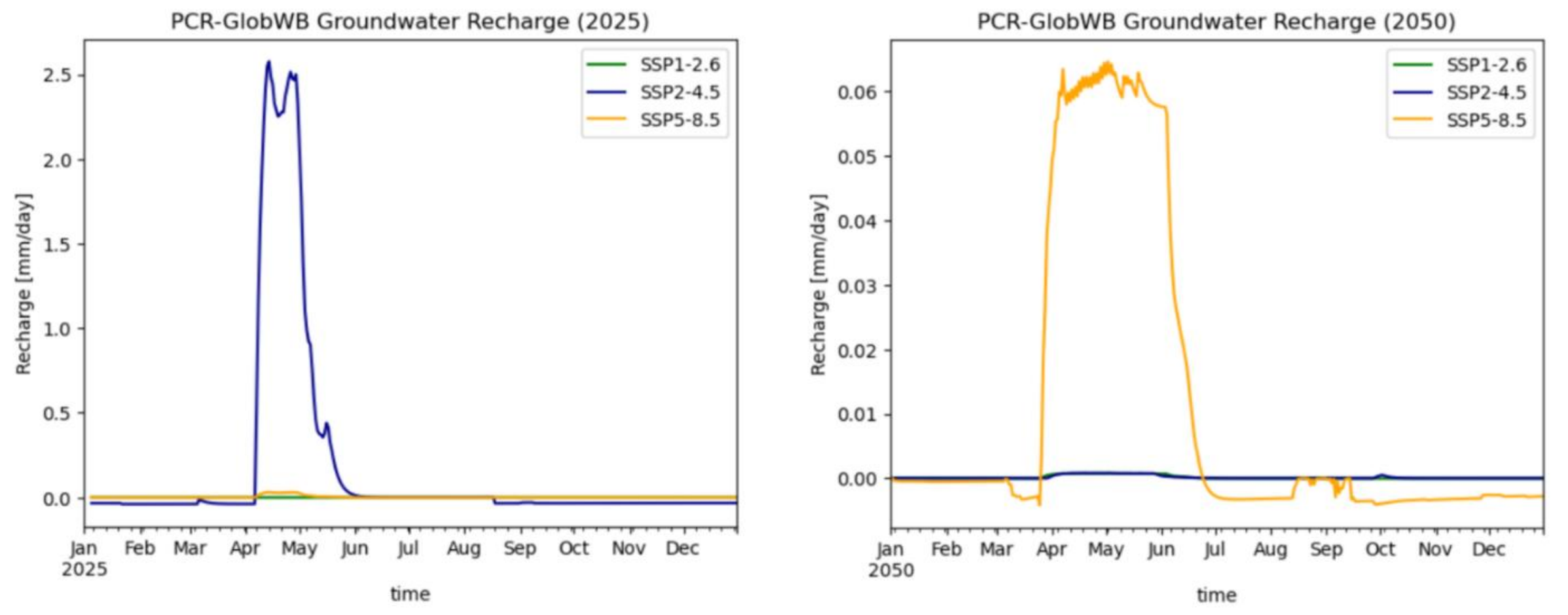Figure 10: PCR-GlobWB simulated groundwater recharge for future climate scenarios for 2025 (left) and 2050 (right).

Simulated Approximation Groundwater Recharge

The simulation of approximated groundwater recharge uses the same forcing dataset and parameter set as described in Section 3.2. Initially, the precipitation, the total evaporation, the total groundwater abstraction, the land surface runoff and the discharge were generated for the period 2025-2100. These components were integrated in the water balance to estimate the approximated groundwater recharge.

Figure 11 illustrates the 21st century divided in two halves, specifically for 2025-2065 and 2065-2100. The century is divided into two halves to improve the clarity of the graph. Appendix E provides a more detailed analysis by dividing graphs into ten-year intervals, offering a more clear visualization of trends within each decade.

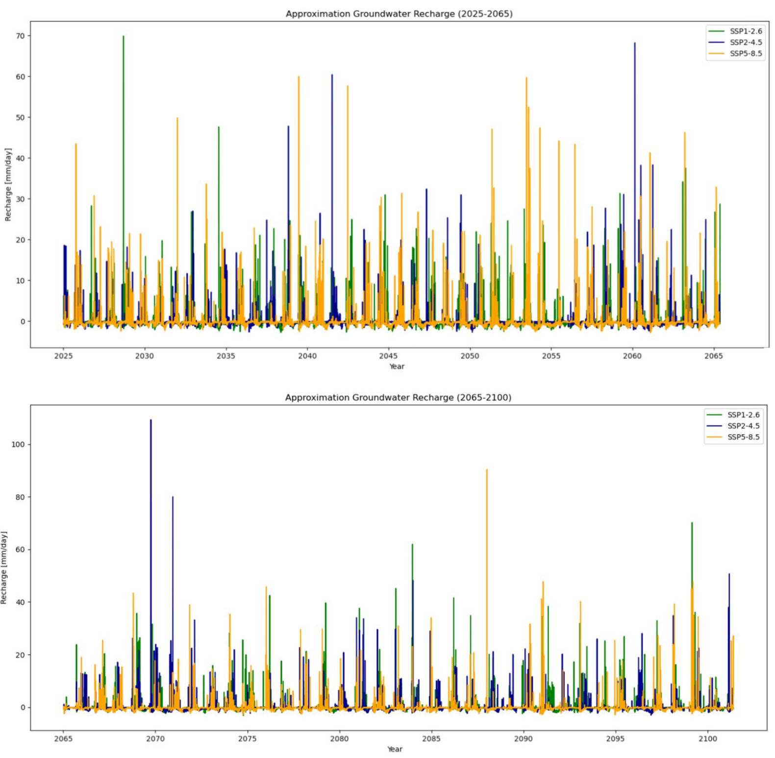Figure 11: Approximated groundwater recharge for 2025-2065 and 2065-2100.

To provide a clearer visual representation of the data depicted in Figure 11, Figure 12 focuses on the years 2025, 2050, 2075 and 2100. These graphs illustrate the approximated groundwater recharge and its seasonal variations. For instance, in 2075, the influence of winter rainfall is evident, with an observed increase during the winter months. Across all highlighted years, it is apparent that the summer season experiences drought conditions.

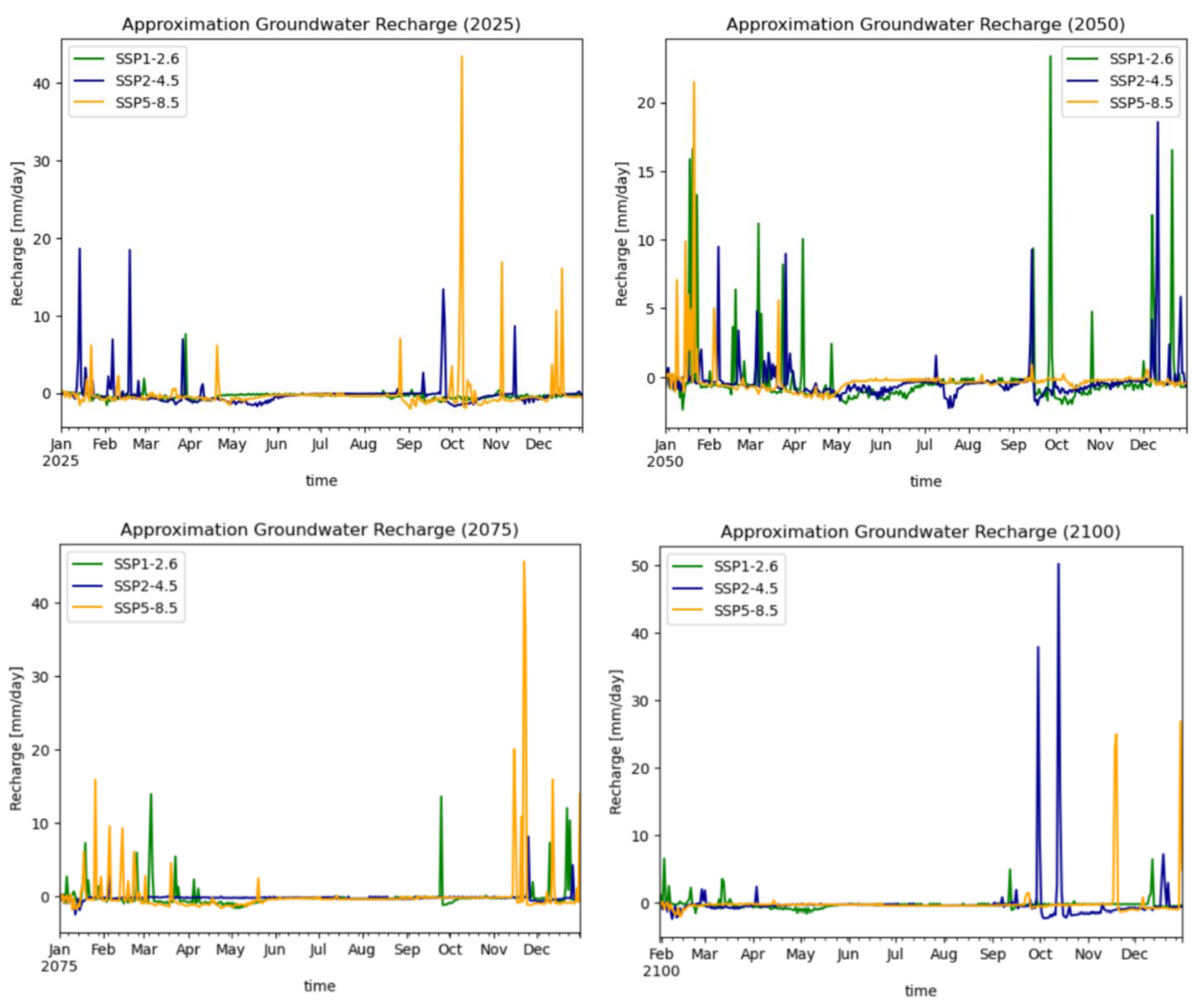Figure 12: Approximated groundwater recharge for the year 2025 (top left), 2050 (top right), 2075 (bottom left) and 2100 (bottom right).

To evaluate the simulated data, Figure 13 presents boxplots summarizing the approximated groundwater recharge for the period 2025-2100. These plots reveal differences in outliers between the climate scenarios. Notably, SSP5-8.5 displays a greater number of outliers ranging between 20 and 50 mm/day. Appendix D includes a Z-value outlier analysis and provides a boxplot without outliers. From this analysis, it is evident that the upper quartile, median and lower quartile display minor differences across the SSPs.

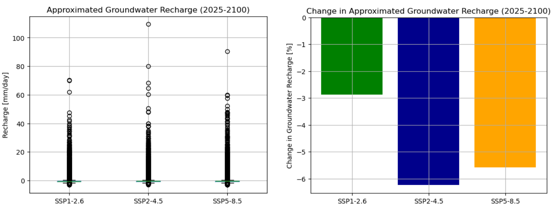Figure 13: (left) Boxplot approximated groundwater recharge for three SSPs (2025-2100). (right) Relative change in approximated groundwater recharge for three SSPs (2025-2100).

The total approximated groundwater recharge for each SSP was determined, and changes were evaluated against the benchmark derived from historical data in Section 3.1. Figure 14 illustrates these changes for the period 2025-2100. Indicating that SSP1-2.6 shows a change of -2.9%, SSP2 4.5 a change of -6.2% and SSP5-8.5 a change of -5.6%. Figure 15 illustrates four diagrams, displaying the changes of near-term, mid-term and long-term periods. The plots are divided into a twenty-year interval (2025-2045, 2045-2065, 2065-2085 and 2085-2100). An overview of the change per SSP is presented in Table 3. This table indicates that the increase in long-term is significantly.

Table 3: change in approximated groundwater recharge per period

Period	SSP1-2.6	SSP2-4.5	SSP5-8.5
2025-2045	\(9.4 \% \)	\(-5.1 \%\)	-\(13.2 \%\)
2045-2065	\(-1.9 \%\)	\(-12.7 \%\)	\(0.7 \%\)
2065-2085	\(-13.7 \% \)	\(-7.3 \%\)	\(-1.3 \%\)
2085-2100	\(-6.2 \% \)	\(2.4 \%\)	\(-9.5 \%\)

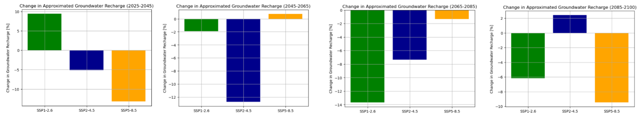Figure 14: Relative change in approximated groundwater recharge for 2025-2045, 2045-2065, 2065-2085 and 2085-2100, relatively shown.