BEP reproduceerbaar verslag#
Deze notebook bevat de belangrijke codes die nodig zijn voor het runnen van de hoofdstuknotebooks.
Belangrijk:
Grote modelruns en het maken van grote
.nc-bestanden staan in codecellen, maar zijn uitgecommentarieerd met#.De lichte cellen lezen bestaande CSV-bestanden in uit
bestanden/en reproduceren de tabellen en figuren.
1. Imports en mappen#
Pas alleen project_dir aan als de projectmap ergens anders staat.
from pathlib import Path

import numpy as np
import pandas as pd
import matplotlib.pyplot as plt

project_dir = Path("/home/niels/BEP-Niels")

repo_dir = project_dir / "book" / "thesis_projects" / "BSc" / "2026_Q4_NielsEijer_CEG"
bestanden_dir = repo_dir / "Bestanden"
rhine_dir = bestanden_dir / "Rhine"

print("Repo map:", repo_dir)
print("Bestandenmap:", bestanden_dir)
print("Bestandenmap bestaat:", bestanden_dir.exists())
print("Rhine map bestaat:", rhine_dir.exists())
Repo map: /home/niels/BEP-Niels/book/thesis_projects/BSc/2026_Q4_NielsEijer_CEG
Bestandenmap: /home/niels/BEP-Niels/book/thesis_projects/BSc/2026_Q4_NielsEijer_CEG/Bestanden
Bestandenmap bestaat: True
Rhine map bestaat: True
2. Bestanden controleren#
Deze cel controleert de kleine bestanden die in GitHub kunnen staan. De grote .nc-bestanden kunnen lokaal worden gemaakt met de uitgecommentarieerde cellen verderop.
required_files = [
    bestanden_dir / "6435060_Q_Day.Cmd.txt",
    bestanden_dir / "lobith_1986_2019_biascorrected.csv",
    bestanden_dir / "lobith_1986_2019_biascor_scores.csv",
    bestanden_dir / "lobith_four_season_qm_relation.csv",
    bestanden_dir / "parametergevoeligheid_scores_1987_1995_tussenstand.csv",
    bestanden_dir / "future_ssp126_2071_2100_lobith_daily_biascorrected.csv",
    bestanden_dir / "future_ssp245_2071_2100_lobith_daily_biascorrected.csv",
    bestanden_dir / "future_ssp585_2071_2100_lobith_daily_biascorrected.csv",
    rhine_dir / "Rhine.shp",
    rhine_dir / "Rhine.dbf",
    rhine_dir / "Rhine.shx",
    rhine_dir / "Rhine.prj",
    rhine_dir / "Rhine.qpj",
]

for file in required_files:
    print(file.name, "bestaat:", file.exists())
6435060_Q_Day.Cmd.txt bestaat: True
lobith_1986_2019_biascorrected.csv bestaat: True
lobith_1986_2019_biascor_scores.csv bestaat: True
lobith_four_season_qm_relation.csv bestaat: True
parametergevoeligheid_scores_1987_1995_tussenstand.csv bestaat: True
future_ssp126_2071_2100_lobith_daily_biascorrected.csv bestaat: True
future_ssp245_2071_2100_lobith_daily_biascorrected.csv bestaat: True
future_ssp585_2071_2100_lobith_daily_biascorrected.csv bestaat: True
Rhine.shp bestaat: True
Rhine.dbf bestaat: True
Rhine.shx bestaat: True
Rhine.prj bestaat: True
Rhine.qpj bestaat: True
3. Hulpfuncties#
Deze functies worden gebruikt voor de tabellen en figuren uit het resultatenhoofdstuk.
def rmse(obs, sim):
    obs = np.asarray(obs)
    sim = np.asarray(sim)
    return np.sqrt(np.mean((sim - obs) ** 2))


def bias(obs, sim):
    obs = np.asarray(obs)
    sim = np.asarray(sim)
    return np.mean(sim - obs)


def log_nse(obs, sim):
    obs = np.asarray(obs)
    sim = np.asarray(sim)

    obs_log = np.log(obs)
    sim_log = np.log(sim)

    teller = np.sum((obs_log - sim_log) ** 2)
    noemer = np.sum((obs_log - obs_log.mean()) ** 2)

    return 1 - teller / noemer


def fdc_values(series):
    values = np.sort(series.dropna().values)[::-1]
    exceedance = np.arange(1, len(values) + 1) / (len(values) + 1) * 100
    return exceedance, values


def add_seasons(data):
    data = data.copy()
    data["month"] = data["date"].dt.month

    data["season"] = "unknown"
    data.loc[data["month"].isin([12, 1, 2]), "season"] = "winter"
    data.loc[data["month"].isin([3, 4, 5]), "season"] = "lente"
    data.loc[data["month"].isin([6, 7, 8]), "season"] = "zomer"
    data.loc[data["month"].isin([9, 10, 11]), "season"] = "herfst"

    return data


def apply_four_season_qm(data, relation_table):
    data = data.copy()
    relation_table = relation_table.copy()

    if "group" in relation_table.columns:
        relation_table = relation_table.rename(columns={"group": "season"})

    data["Q_model_biascorrected_m3s"] = np.nan

    for season in ["winter", "lente", "zomer", "herfst"]:
        season_relation = relation_table[relation_table["season"] == season].copy()
        season_relation = season_relation.sort_values("model_q")

        model_q = season_relation["model_q"].values
        grdc_q = season_relation["grdc_q"].values

        mask = data["season"] == season

        data.loc[mask, "Q_model_biascorrected_m3s"] = np.interp(
            data.loc[mask, "Q_model_raw_m3s"],
            model_q,
            grdc_q
        )

    return data


def find_lowflow_events(data, discharge_col, threshold):
    data = data.copy().sort_values("date")
    data["below_threshold"] = data[discharge_col] < threshold

    events = []
    current_start = None
    current_length = 0
    previous_date = None

    for _, row in data.iterrows():
        if row["below_threshold"]:
            if current_start is None:
                current_start = row["date"]
                current_length = 1
            else:
                current_length += 1
        else:
            if current_start is not None:
                events.append({
                    "start_date": current_start,
                    "end_date": previous_date,
                    "duration_days": current_length
                })
                current_start = None
                current_length = 0

        previous_date = row["date"]

    if current_start is not None:
        events.append({
            "start_date": current_start,
            "end_date": previous_date,
            "duration_days": current_length
        })

    return pd.DataFrame(events)
4. Historische biascorrectie: invoerbestanden#
Deze bestanden zijn afkomstig uit de historische kalibratie- en biascorrectienotebooks. De four-season kolom is de methode die in het verslag is gebruikt.
historical_file = bestanden_dir / "lobith_1986_2019_biascorrected.csv"
scores_file = bestanden_dir / "lobith_1986_2019_biascor_scores.csv"
relation_file = bestanden_dir / "lobith_four_season_qm_relation.csv"

historical = pd.read_csv(historical_file)
historical["date"] = pd.to_datetime(historical["date"])

bias_scores = pd.read_csv(scores_file)
four_relation = pd.read_csv(relation_file)

print(historical.columns.tolist())
display(historical.head())
display(bias_scores.head())
display(four_relation.head())
['date', 'Q_grdc_m3s', 'Q_model_raw_m3s', 'Q_model_annual_fdc_m3s', 'Q_model_two_season_fdc_m3s', 'Q_model_four_season_fdc_m3s', 'month', 'two_season', 'four_season']
| date | Q_grdc_m3s | Q_model_raw_m3s | Q_model_annual_fdc_m3s | Q_model_two_season_fdc_m3s | Q_model_four_season_fdc_m3s | month | two_season | four_season | |
|---|---|---|---|---|---|---|---|---|---|
| 0 | 1987-01-01 | 4865.0 | 12101.763672 | 6976.499195 | 7302.245563 | 6644.466539 | 1 | jan_jun | winter |
| 1 | 1987-01-02 | 5756.0 | 13396.190430 | 7725.032013 | 8260.342483 | 7565.702692 | 1 | jan_jun | winter |
| 2 | 1987-01-03 | 6160.0 | 14481.406250 | 8267.416049 | 9138.001682 | 8498.884130 | 1 | jan_jun | winter |
| 3 | 1987-01-04 | 6973.0 | 14916.130859 | 8484.688672 | 9489.581566 | 8702.814537 | 1 | jan_jun | winter |
| 4 | 1987-01-05 | 7579.0 | 14704.667969 | 8379.000850 | 9318.562725 | 8603.906462 | 1 | jan_jun | winter |
| period | run | bias | rmse | log_nse | diff_days_below_1600 | diff_days_below_1020 | diff_p10 | diff_p17 | n_days | perc_days | |
|---|---|---|---|---|---|---|---|---|---|---|---|
| 0 | calibration_1987_2003 | calib10_raw | 1149.77 | 2089.22 | -0.60 | -300 | 572 | -293.09 | -125.60 | 6209 | 9.21 |
| 1 | calibration_1987_2003 | annual_fdc | 0.68 | 686.27 | 0.61 | 9 | -3 | -0.00 | 0.07 | 6209 | -0.05 |
| 2 | calibration_1987_2003 | two_season_fdc | 1.81 | 585.60 | 0.71 | 7 | 4 | 3.21 | 4.02 | 6209 | 0.06 |
| 3 | calibration_1987_2003 | four_season_fdc | 0.29 | 575.73 | 0.73 | 6 | 3 | 2.28 | 1.75 | 6209 | 0.05 |
| 4 | validation_2004_2019 | calib10_raw | 1130.10 | 1943.32 | -1.22 | -434 | 533 | -326.08 | -117.06 | 5844 | 9.12 |
| season | quantile | model_q | grdc_q | |
|---|---|---|---|---|
| 0 | winter | 0.00 | 378.058990 | 855.00 |
| 1 | winter | 0.01 | 489.880028 | 933.65 |
| 2 | winter | 0.02 | 573.746072 | 1052.62 |
| 3 | winter | 0.03 | 671.807537 | 1098.98 |
| 4 | winter | 0.04 | 744.721763 | 1127.32 |
5. Tabel 4.2 - Prestatie-indicatoren four-season biascorrectie#
Deze tabel wordt direct uit lobith_1986_2019_biascor_scores.csv gehaald. In het verslag is de run four_season_fdc gebruikt.
period_labels = {
    "calibration_1987_2003": "Kalibratie 1987-2003",
    "validation_2004_2019": "Validatie 2004-2019",
    "validation_2004_2010": "Validatie 2004-2010",
    "validation_2011_2019": "Validatie 2011-2019",
}

selected_periods = list(period_labels.keys())

tabel_4_2 = bias_scores[
    (bias_scores["run"] == "four_season_fdc") &
    (bias_scores["period"].isin(selected_periods))
].copy()

tabel_4_2["Periode"] = tabel_4_2["period"].map(period_labels)

tabel_4_2 = tabel_4_2[[
    "Periode",
    "bias",
    "rmse",
    "log_nse",
    "diff_days_below_1020",
    "diff_days_below_1600"
]].rename(columns={
    "bias": "Bias (m3/s)",
    "rmse": "RMSE (m3/s)",
    "log_nse": "Log-NSE",
    "diff_days_below_1020": "Diff. < 1020 (d)",
    "diff_days_below_1600": "Diff. < 1600 (d)",
})

tabel_4_2
| Periode | Bias (m3/s) | RMSE (m3/s) | Log-NSE | Diff. < 1020 (d) | Diff. < 1600 (d) | |
|---|---|---|---|---|---|---|
| 3 | Kalibratie 1987-2003 | 0.29 | 575.73 | 0.73 | 3 | 6 |
| 7 | Validatie 2004-2019 | 125.91 | 557.78 | 0.66 | 43 | -131 |
| 11 | Validatie 2004-2010 | 179.80 | 549.45 | 0.54 | 54 | -150 |
| 15 | Validatie 2011-2019 | 83.99 | 564.18 | 0.73 | -11 | 19 |
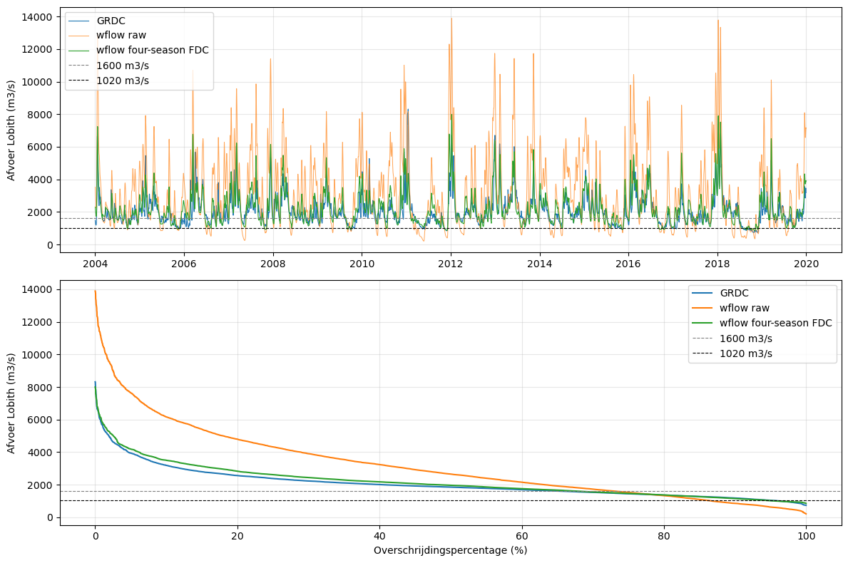
6. Figuur 4.1 - Validatieperiode 2004-2019#
Deze figuur gebruikt dezelfde kolommen als in de historische biascorrectie-output.
validation = historical[
    (historical["date"] >= "2004-01-01") &
    (historical["date"] <= "2019-12-31")
].copy()

fig, axes = plt.subplots(2, 1, figsize=(12, 8))

axes[0].plot(validation["date"], validation["Q_grdc_m3s"], label="GRDC", linewidth=0.8)
axes[0].plot(validation["date"], validation["Q_model_raw_m3s"], label="wflow raw", linewidth=0.7, alpha=0.7)
axes[0].plot(validation["date"], validation["Q_model_four_season_fdc_m3s"], label="wflow four-season FDC", linewidth=0.8)
axes[0].axhline(1600, linestyle="--", color="grey", linewidth=0.8, label="1600 m3/s")
axes[0].axhline(1020, linestyle="--", color="black", linewidth=0.8, label="1020 m3/s")
axes[0].set_ylabel("Afvoer Lobith (m3/s)")
axes[0].grid(True, alpha=0.3)
axes[0].legend()

for label, col in {
    "GRDC": "Q_grdc_m3s",
    "wflow raw": "Q_model_raw_m3s",
    "wflow four-season FDC": "Q_model_four_season_fdc_m3s",
}.items():
    x, y = fdc_values(validation[col])
    axes[1].plot(x, y, label=label)

axes[1].axhline(1600, linestyle="--", color="grey", linewidth=0.8, label="1600 m3/s")
axes[1].axhline(1020, linestyle="--", color="black", linewidth=0.8, label="1020 m3/s")
axes[1].set_xlabel("Overschrijdingspercentage (%)")
axes[1].set_ylabel("Afvoer Lobith (m3/s)")
axes[1].grid(True, alpha=0.3)
axes[1].legend()

plt.tight_layout()
plt.show()
7. CMIP delta-change en future forcing maken#
De grote .nc-bestanden worden niet op GitHub gezet. Deze uitgecommentarieerde cel documenteert hoe ze in 019_CMIP_ERA5 zijn gemaakt.
Belangrijke lijn uit de oorspronkelijke notebooks:
ds_forcingkomt uittemp_runs/calib10_long_1986_2019, uit het.nc-bestand metpr,tasenpet.De monthly climate signals staan in
results/CMIP_delta_change.Voor de uiteindelijke wflow-runs wordt spin-up gebruikt: 2069-2100, analyse vanaf 2071.
# import xarray as xr
#
# run_dir = temp_dir / "calib10_long_1986_2019"
# nc_files = list(run_dir.rglob("*.nc"))
#
# forcing_file = None
# for file in nc_files:
#     try:
#         ds = xr.open_dataset(file)
#         vars_in_file = list(ds.data_vars)
#         ds.close()
#
#         if ("pr" in vars_in_file) and ("tas" in vars_in_file) and ("pet" in vars_in_file):
#             forcing_file = file
#             break
#     except Exception:
#         pass
#
# ds_forcing = xr.open_dataset(forcing_file)
#
# climate_signals_wflow_grid = {}
# for scenario in ["ssp126", "ssp245", "ssp585"]:
#     climate_signals_wflow_grid[scenario] = xr.open_dataset(
#         cmip_dir / f"{scenario}_monthly_climate_signal_wflow_grid.nc"
#     )
#
# def apply_climate_signal_to_forcing(base_forcing, signal, future_start_date):
#     months = xr.DataArray(
#         base_forcing["time"].dt.month.values,
#         dims="time",
#         coords={"time": base_forcing.time}
#     )
#
#     pr_factor = signal["pr_factor"].sel(month=months)
#     tas_delta = signal["tas_delta"].sel(month=months)
#
#     pr_future = base_forcing["pr"] * pr_factor
#     tas_future = base_forcing["tas"] + tas_delta
#     pet_future = base_forcing["pet"]
#
#     future_times = pd.date_range(
#         start=future_start_date,
#         periods=len(base_forcing.time),
#         freq="D"
#     ) + pd.Timedelta(hours=12)
#
#     future_forcing = xr.Dataset({
#         "pr": pr_future,
#         "tas": tas_future,
#         "pet": pet_future
#     })
#
#     future_forcing = future_forcing.assign_coords(
#         time=future_times,
#         lat=base_forcing.lat,
#         lon=base_forcing.lon
#     )
#
#     future_forcing = future_forcing.drop_vars("month", errors="ignore")
#     future_forcing["pr"] = future_forcing["pr"].clip(min=0)
#
#     future_forcing["pr"].attrs = base_forcing["pr"].attrs
#     future_forcing["tas"].attrs = base_forcing["tas"].attrs
#     future_forcing["pet"].attrs = base_forcing["pet"].attrs
#
#     return future_forcing
#
# future_temp_forcing_dir = temp_dir / "future_forcing_spinup"
# future_temp_forcing_dir.mkdir(parents=True, exist_ok=True)
#
# spinup_base_forcing = ds_forcing.sel(time=slice("1988-01-01", "2019-12-31"))
#
# def create_spinup_future_forcing_file(scenario):
#     signal = climate_signals_wflow_grid[scenario]
#
#     future_forcing = apply_climate_signal_to_forcing(
#         base_forcing=spinup_base_forcing,
#         signal=signal,
#         future_start_date="2069-01-01"
#     )
#
#     future_forcing = future_forcing.sel(time=slice("2069-01-01", "2100-12-31"))
#
#     output_file = future_temp_forcing_dir / f"wflow_forcing_{scenario}_2069_2100_uncompressed.nc"
#
#     encoding = {
#         "pr": {"dtype": "float32"},
#         "tas": {"dtype": "float32"},
#         "pet": {"dtype": "float32"}
#     }
#
#     future_forcing.to_netcdf(output_file, encoding=encoding)
#     future_forcing.close()
#
#     print("Opgeslagen als:", output_file)
#     return output_file
#
# for scenario in ["ssp126", "ssp245", "ssp585"]:
#     create_spinup_future_forcing_file(scenario)
8. Toekomstige wflow-runs uitvoeren#
Deze cel komt overeen met 020_SSP126, 021_SSP245 en 022_SSP585. De code staat uit, zodat de runs niet per ongeluk starten.
# import shutil
# from ewatercycle.models import Wflow
# from ewatercycle.parameter_sets import available_parameter_sets
# from ewatercycle.forcing import sources
#
# analysis_start = "2071-01-01"
# analysis_end = "2100-12-31"
# lat_lobith = 51.85
# lon_lobith = 6.10
#
# parameter_factors = {
#     "CanopyGapFraction.tbl": 1.25,
#     "N_River.tbl": 2.00,
#     "N.tbl": 1.25
# }
#
# def multiply_tbl_last_column(tbl_file, factor):
#     tbl_file = Path(tbl_file)
#     lines = tbl_file.read_text().splitlines()
#     new_lines = []
#
#     for line in lines:
#         stripped = line.strip()
#         if stripped == "" or stripped.startswith("#"):
#             new_lines.append(line)
#             continue
#
#         parts = line.split()
#         try:
#             old_value = float(parts[-1])
#             parts[-1] = str(old_value * factor)
#             new_lines.append(" ".join(parts))
#         except:
#             new_lines.append(line)
#
#     tbl_file.write_text("\n".join(new_lines) + "\n")
#
# def apply_parameter_factors(cfg_dir, parameter_factors):
#     cfg_dir = Path(cfg_dir)
#     for tbl_name, factor in parameter_factors.items():
#         tbl_files = list(cfg_dir.rglob(tbl_name))
#         for tbl_file in tbl_files:
#             multiply_tbl_last_column(tbl_file, factor)
#
# parameter_sets = available_parameter_sets(target_model="wflow")
# parameter_set = parameter_sets["wflow_rhine_sbm_nc"]
# WflowForcing = sources["WflowForcing"]
# shape_file = project_dir / "Rhine" / "Rhine.shp"
#
# def run_future_wflow_scenario(scenario):
#     future_forcing_file = temp_dir / "future_forcing_spinup" / f"wflow_forcing_{scenario}_2069_2100_uncompressed.nc"
#
#     future_wflow_forcing = WflowForcing(
#         start_time="2069-01-01T00:00:00Z",
#         end_time="2101-01-01T00:00:00Z",
#         directory=str(future_forcing_file.parent),
#         shape=str(shape_file),
#         netcdfinput=future_forcing_file.name,
#         Precipitation="/pr",
#         EvapoTranspiration="/pet",
#         Temperature="/tas",
#         Inflow=None,
#     )
#
#     run_name = f"future_{scenario}_2069_2100"
#     cfg_dir_run = temp_dir / f"run_{run_name}"
#
#     if cfg_dir_run.exists():
#         shutil.rmtree(cfg_dir_run)
#
#     model = Wflow(parameter_set=parameter_set, forcing=future_wflow_forcing)
#     cfg_file, cfg_dir = model.setup(cfg_dir=str(cfg_dir_run))
#     cfg_dir = Path(cfg_dir)
#
#     apply_parameter_factors(cfg_dir, parameter_factors)
#     model.initialize(cfg_file)
#
#     q_values = []
#     times = []
#     step = 0
#
#     while model.time < model.end_time:
#         model.update()
#
#         q_lobith = model.get_value_at_coords(
#             "RiverRunoff",
#             lat=[lat_lobith],
#             lon=[lon_lobith]
#         )[0]
#
#         q_values.append(float(q_lobith))
#         times.append(model.time_as_datetime)
#         step += 1
#
#         if step % 365 == 0:
#             print("Stap:", step, "Tijd:", model.time_as_datetime, "Q Lobith:", round(float(q_lobith), 1))
#
#     model.finalize()
#
#     output = pd.DataFrame({
#         "date": pd.to_datetime(times, utc=True),
#         "Q_model_raw_m3s": q_values
#     })
#
#     output["date"] = output["date"].dt.tz_convert(None).dt.floor("D")
#
#     full_output_file = results_dir / f"future_{scenario}_2069_2100_lobith_daily_full.csv"
#     output.to_csv(full_output_file, index=False)
#
#     analysis_output = output[
#         (output["date"] >= pd.to_datetime(analysis_start)) &
#         (output["date"] <= pd.to_datetime(analysis_end))
#     ].copy()
#
#     raw_output_file = results_dir / f"future_{scenario}_2071_2100_lobith_daily_raw.csv"
#     analysis_output.to_csv(raw_output_file, index=False)
#
#     return output, analysis_output
#
# for scenario in ["ssp126", "ssp245", "ssp585"]:
#     run_future_wflow_scenario(scenario)
9. Four-season biascorrectie toepassen op scenario-output#
Als de ruwe scenario-output opnieuw wordt gemaakt, kan deze cel de four-season biascorrectie opnieuw toepassen en dezelfde eindbestanden maken die in 023 en 024 zijn gebruikt.
# for scenario in ["ssp126", "ssp245", "ssp585"]:
#     raw_output_file = results_dir / f"future_{scenario}_2071_2100_lobith_daily_raw.csv"
#     biascorrected_output_file = results_dir / f"future_{scenario}_2071_2100_lobith_daily_biascorrected.csv"
#
#     future_raw = pd.read_csv(raw_output_file)
#     future_raw["date"] = pd.to_datetime(future_raw["date"])
#
#     if "Q_model_raw_m3s" not in future_raw.columns:
#         future_raw = future_raw.rename(columns={"Q_model_m3s": "Q_model_raw_m3s"})
#
#     future_raw = future_raw[
#         (future_raw["date"] >= "2071-01-01") &
#         (future_raw["date"] <= "2100-12-31")
#     ].copy()
#
#     future_raw = future_raw[["date", "Q_model_raw_m3s"]].copy()
#     future_corrected = add_seasons(future_raw)
#     future_corrected = apply_four_season_qm(future_corrected, four_relation)
#
#     future_corrected.to_csv(biascorrected_output_file, index=False)
#     print("Opgeslagen als:", biascorrected_output_file)
10. Scenario-output inlezen#
Deze drie bestanden zijn de eindbestanden uit 020, 021 en 022. Ze zijn klein genoeg om in de publicatiemap te bewaren.
future_files = {
    "ssp126": bestanden_dir / "future_ssp126_2071_2100_lobith_daily_biascorrected.csv",
    "ssp245": bestanden_dir / "future_ssp245_2071_2100_lobith_daily_biascorrected.csv",
    "ssp585": bestanden_dir / "future_ssp585_2071_2100_lobith_daily_biascorrected.csv",
}

future_data_list = []

for scenario, file in future_files.items():
    data = pd.read_csv(file)
    data["date"] = pd.to_datetime(data["date"])
    data["scenario"] = scenario

    data = data[
        (data["date"] >= "2071-01-01") &
        (data["date"] <= "2100-12-31")
    ].copy()

    future_data_list.append(data)

scenario_data = pd.concat(future_data_list, ignore_index=True)

scenario_data.groupby("scenario").agg(
    start=("date", "min"),
    end=("date", "max"),
    n_days=("date", "count"),
    q5=("Q_model_biascorrected_m3s", lambda x: x.quantile(0.05)),
    q10=("Q_model_biascorrected_m3s", lambda x: x.quantile(0.10)),
)
| start | end | n_days | q5 | q10 | |
|---|---|---|---|---|---|
| scenario | |||||
| ssp126 | 2071-01-01 | 2100-12-31 | 10957 | 1038.222141 | 1160.978964 |
| ssp245 | 2071-01-01 | 2100-12-31 | 10957 | 968.810322 | 1083.762324 |
| ssp585 | 2071-01-01 | 2100-12-31 | 10957 | 945.006031 | 1040.219441 |
11. Tabel 4.3 - Lage-afvoerpercentielen en kritieke dagen#
Deze cel reproduceert Tabel 4.3 uit het verslag.
historical_start = "1990-01-01"
historical_end = "2019-12-31"
future_start = "2071-01-01"
future_end = "2100-12-31"
thresholds = [1020, 1133, 1229]

scenario_labels = {
    "ssp126": "SSP1-2.6 2071-2100",
    "ssp245": "SSP2-4.5 2071-2100",
    "ssp585": "SSP5-8.5 2071-2100",
}

historical_grdc = historical[
    (historical["date"] >= historical_start) &
    (historical["date"] <= historical_end)
].copy()

historical_grdc = historical_grdc[["date", "Q_grdc_m3s"]].rename(
    columns={"Q_grdc_m3s": "Q_m3s"}
)
historical_grdc["scenario"] = "Historisch GRDC 1990-2019"

future_rows = []

for scenario, file in future_files.items():
    data = pd.read_csv(file)
    data["date"] = pd.to_datetime(data["date"])

    data = data[
        (data["date"] >= future_start) &
        (data["date"] <= future_end)
    ].copy()

    data = data[["date", "Q_model_biascorrected_m3s"]].rename(
        columns={"Q_model_biascorrected_m3s": "Q_m3s"}
    )

    data["scenario"] = scenario_labels[scenario]
    future_rows.append(data)

future_all = pd.concat(future_rows, ignore_index=True)
table_data = pd.concat([historical_grdc, future_all], ignore_index=True)

rows = []

for scenario in table_data["scenario"].unique():
    scenario_data = table_data[table_data["scenario"] == scenario].copy()
    n_years = scenario_data["date"].dt.year.nunique()

    row = {
        "Scenario": scenario,
        "q5 (m3/s)": round(scenario_data["Q_m3s"].quantile(0.05)),
        "q10 (m3/s)": round(scenario_data["Q_m3s"].quantile(0.10)),
        "OLA 1020 (d/jr)": round((scenario_data["Q_m3s"] < 1020).sum() / n_years, 1),
        "10%-scen. 1133 (d/jr)": round((scenario_data["Q_m3s"] < 1133).sum() / n_years, 1),
        "17%-scen. 1229 (d/jr)": round((scenario_data["Q_m3s"] < 1229).sum() / n_years, 1),
    }

    rows.append(row)

tabel_4_3 = pd.DataFrame(rows)
tabel_4_3
| Scenario | q5 (m3/s) | q10 (m3/s) | OLA 1020 (d/jr) | 10%-scen. 1133 (d/jr) | 17%-scen. 1229 (d/jr) | |
|---|---|---|---|---|---|---|
| 0 | Historisch GRDC 1990-2019 | 1057 | 1185 | 14.3 | 28.2 | 43.4 |
| 1 | SSP1-2.6 2071-2100 | 1038 | 1161 | 15.8 | 32.6 | 45.0 |
| 2 | SSP2-4.5 2071-2100 | 969 | 1084 | 27.4 | 46.8 | 62.7 |
| 3 | SSP5-8.5 2071-2100 | 945 | 1040 | 33.5 | 54.2 | 70.1 |
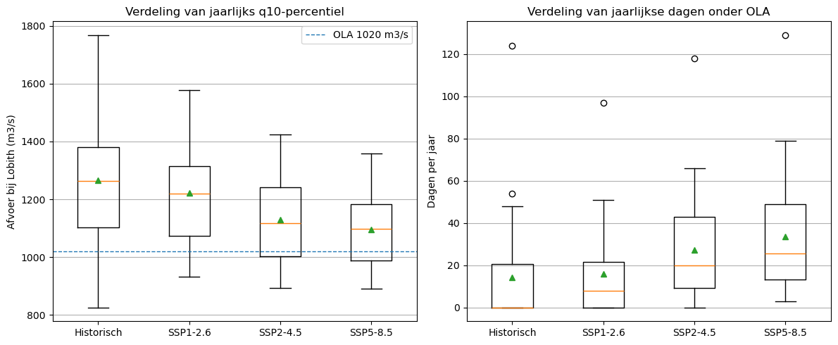
12. Figuur 4.2 - Boxplots jaarlijkse q10 en dagen onder OLA#
Deze figuur volgt de aanpak uit 023_scenario_vergelijkingen: jaarlijkse indicatoren worden berekend uit GRDC en de drie biasgecorrigeerde scenario-outputbestanden.
ola_threshold = 1020

# Historische jaarlijkse indicatoren
annual_hist = historical_grdc.copy()
annual_hist["year"] = annual_hist["date"].dt.year
annual_hist = annual_hist.groupby("year").agg(
    q10_annual=("Q_m3s", lambda x: x.quantile(0.10)),
    days_below_ola=("Q_m3s", lambda x: (x < ola_threshold).sum())
).reset_index()
annual_hist["scenario"] = "Historisch"
annual_hist["period_year"] = annual_hist["year"] - annual_hist["year"].min() + 1

# Toekomstige jaarlijkse indicatoren
future_for_annual = future_all.copy()
future_for_annual["year"] = future_for_annual["date"].dt.year

annual_future = future_for_annual.groupby(["scenario", "year"]).agg(
    q10_annual=("Q_m3s", lambda x: x.quantile(0.10)),
    days_below_ola=("Q_m3s", lambda x: (x < ola_threshold).sum())
).reset_index()

annual_future["scenario"] = annual_future["scenario"].replace({
    "SSP1-2.6 2071-2100": "SSP1-2.6",
    "SSP2-4.5 2071-2100": "SSP2-4.5",
    "SSP5-8.5 2071-2100": "SSP5-8.5",
})

annual_future["period_year"] = annual_future.groupby("scenario")["year"].transform(
    lambda x: x - x.min() + 1
)

annual_all = pd.concat([annual_hist, annual_future], ignore_index=True)

plot_order = ["Historisch", "SSP1-2.6", "SSP2-4.5", "SSP5-8.5"]
q10_data = []
days_data = []

for name in plot_order:
    data = annual_all[annual_all["scenario"] == name]
    q10_data.append(data["q10_annual"])
    days_data.append(data["days_below_ola"])

fig, axes = plt.subplots(1, 2, figsize=(12, 5))

axes[0].boxplot(q10_data, labels=plot_order, showmeans=True)
axes[0].axhline(1020, linestyle="--", linewidth=1, label="OLA 1020 m3/s")
axes[0].set_title("Verdeling van jaarlijks q10-percentiel")
axes[0].set_ylabel("Afvoer bij Lobith (m3/s)")
axes[0].grid(True, axis="y")
axes[0].legend()

axes[1].boxplot(days_data, labels=plot_order, showmeans=True)
axes[1].set_title("Verdeling van jaarlijkse dagen onder OLA")
axes[1].set_ylabel("Dagen per jaar")
axes[1].grid(True, axis="y")

plt.tight_layout()
plt.show()
13. Tabel 4.4 - Aaneengesloten kritieke laagwaterperioden#
Deze cel reproduceert Tabel 4.4 uit het verslag.
threshold = 1020

event_summary_rows = []
all_events = []

# Historische GRDC 1990-2019
historical_events = find_lowflow_events(
    data=historical_grdc,
    discharge_col="Q_m3s",
    threshold=threshold
)

historical_events["Scenario"] = "Historisch GRDC 1990-2019"
all_events.append(historical_events)

event_summary_rows.append({
    "Scenario": "Historisch GRDC 1990-2019",
    "Aantal events": len(historical_events),
    "Gem. (d)": round(historical_events["duration_days"].mean(), 1),
    "Mediaan (d)": historical_events["duration_days"].median(),
    "Max. (d)": int(historical_events["duration_days"].max())
})

# Toekomstscenario's 2071-2100
for scenario in ["SSP1-2.6 2071-2100", "SSP2-4.5 2071-2100", "SSP5-8.5 2071-2100"]:
    future_scenario = future_all[future_all["scenario"] == scenario].copy()

    future_events = find_lowflow_events(
        data=future_scenario,
        discharge_col="Q_m3s",
        threshold=threshold
    )

    future_events["Scenario"] = scenario
    all_events.append(future_events)

    event_summary_rows.append({
        "Scenario": scenario,
        "Aantal events": len(future_events),
        "Gem. (d)": round(future_events["duration_days"].mean(), 1),
        "Mediaan (d)": future_events["duration_days"].median(),
        "Max. (d)": int(future_events["duration_days"].max())
    })

tabel_4_4 = pd.DataFrame(event_summary_rows)
tabel_4_4
| Scenario | Aantal events | Gem. (d) | Mediaan (d) | Max. (d) | |
|---|---|---|---|---|---|
| 0 | Historisch GRDC 1990-2019 | 35 | 12.3 | 8.0 | 86 |
| 1 | SSP1-2.6 2071-2100 | 34 | 13.9 | 9.5 | 51 |
| 2 | SSP2-4.5 2071-2100 | 52 | 15.8 | 10.0 | 55 |
| 3 | SSP5-8.5 2071-2100 | 57 | 17.6 | 12.0 | 120 |
14. Appendix A - Parametergevoeligheid#
Deze tabel gebruikt de aangeleverde tussenstand van de parametergevoeligheidstest.
parameter_file = bestanden_dir / "parametergevoeligheid_scores_1987_1995_tussenstand.csv"
parametergevoeligheid = pd.read_csv(parameter_file)
parametergevoeligheid
| run_name | file | bias | rmse | log_nse | bias_low_1600 | mae_low_1600 | grdc_days_below_1600 | model_days_below_1600 | diff_days_below_1600 | grdc_days_below_1020 | model_days_below_1020 | diff_days_below_1020 | grdc_p10 | model_p10 | diff_p10 | grdc_p17 | model_p17 | diff_p17 | |
|---|---|---|---|---|---|---|---|---|---|---|---|---|---|---|---|---|---|---|---|
| 0 | sens_FirstZoneCapacity_x1p25 | sens_FirstZoneCapacity_x1p25_lobith_daily.csv | 710.10 | 1998.63 | -0.94 | -116.22 | 575.02 | 1150 | 1291 | 141 | 125 | 812 | 687 | 1187.2 | 572.26 | -614.94 | 1310.62 | 779.24 | -531.38 |
| 1 | sens_FirstZoneKsatVer_x0p75 | sens_FirstZoneKsatVer_x0p75_lobith_daily.csv | 710.10 | 1998.63 | -0.94 | -116.22 | 575.02 | 1150 | 1291 | 141 | 125 | 812 | 687 | 1187.2 | 572.26 | -614.94 | 1310.62 | 779.24 | -531.38 |
| 2 | sens_InfiltCapSoil_x1p25 | sens_InfiltCapSoil_x1p25_lobith_daily.csv | 710.10 | 1998.63 | -0.94 | -116.22 | 575.02 | 1150 | 1291 | 141 | 125 | 812 | 687 | 1187.2 | 572.26 | -614.94 | 1310.62 | 779.24 | -531.38 |
| 3 | sens_MaxCanopyStorage_x0p75 | sens_MaxCanopyStorage_x0p75_lobith_daily.csv | 721.40 | 2005.52 | -0.93 | -108.78 | 575.95 | 1150 | 1284 | 134 | 125 | 804 | 679 | 1187.2 | 576.41 | -610.79 | 1310.62 | 783.59 | -527.03 |
| 4 | sens_N_Floodplain_x1p25 | sens_N_Floodplain_x1p25_lobith_daily.csv | 710.10 | 1998.63 | -0.94 | -116.22 | 575.02 | 1150 | 1291 | 141 | 125 | 812 | 687 | 1187.2 | 572.26 | -614.94 | 1310.62 | 779.24 | -531.38 |
| 5 | sens_N_River_x1p25 | sens_N_River_x1p25_lobith_daily.csv | 709.76 | 1912.76 | -0.79 | -90.25 | 551.86 | 1150 | 1265 | 115 | 125 | 780 | 655 | 1187.2 | 609.42 | -577.78 | 1310.62 | 811.16 | -499.46 |
| 6 | sens_N_x1p25 | sens_N_x1p25_lobith_daily.csv | 709.75 | 1949.19 | -0.81 | -104.22 | 558.28 | 1150 | 1272 | 122 | 125 | 795 | 670 | 1187.2 | 600.21 | -586.99 | 1310.62 | 807.94 | -502.68 |
| 7 | sens_PET_x0p90 | sens_PET_x0p90_lobith_daily.csv | 987.99 | 2256.18 | -0.95 | 55.32 | 635.29 | 1150 | 1121 | -29 | 125 | 692 | 567 | 1187.2 | 648.40 | -538.80 | 1310.62 | 879.59 | -431.03 |
| 8 | sens_PET_x0p95 | sens_PET_x0p95_lobith_daily.csv | 847.86 | 2126.10 | -0.93 | -33.91 | 598.95 | 1150 | 1211 | 61 | 125 | 757 | 632 | 1187.2 | 603.01 | -584.19 | 1310.62 | 830.79 | -479.83 |
| 9 | sens_RootingDepth_x0p75 | sens_RootingDepth_x0p75_lobith_daily.csv | 731.00 | 2024.48 | -0.95 | -103.10 | 581.15 | 1150 | 1281 | 131 | 125 | 804 | 679 | 1187.2 | 577.05 | -610.15 | 1310.62 | 784.62 | -526.00 |